07-11-2026


|
Getting your Trinity Audio player ready...
|
This post was first published on Medium.
Copy Constraints
In Part 1, we have explained how to transform a computation one wants to prove using PLONK into an intermediate constraint system, which is eventually proved using a Polynomial Commitment Scheme (PCS). We have only covered one type of constraints: gate constraints. In this article, we cover the other type: copy constraints.
Copy constraints
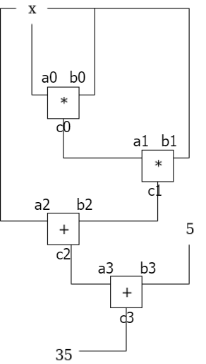
In Part 1, we have enforced constraints within each gate, e.g., a0 * b0 = c0. However, there are also constraints across different gates, e.g., the output of gate 0 is the left input of gate 1, thus c0 = a1. In addition, a wire can be split, e.g., a0 = b0 = b1 = a2. These constraints are called copy constraints to ensure wires contain same value.
Permutation check
Let us first consider copy constraints within a single vector (i.e., a single polynomial), say, a0 = a2.
We define a permutation function σ. σ(i) is the new index of the i-th element in the permuted vector. In our case, σ = (2, 1, 0, 3) as Fig. 2 shows, meaning a0 and a2 switch place.
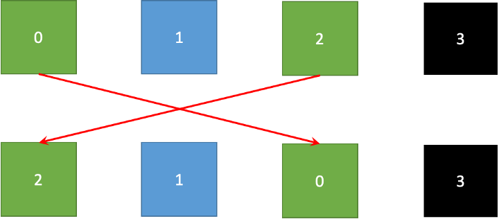
Color represents wire value in the figure. If permuted blocks have same color as the original blocks at the top, copy constraints are met.
Grand product
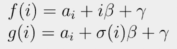
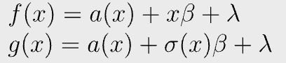
Let us choose two random numbers β and γ. Define f and g as:
Permutation check passes if and only if the following equation holds:
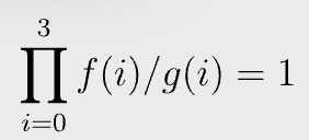
The left hand side is called a grand product. In our concrete example, it is trivial to see the equation holds when a0 = a2, since all the terms in the numerator and denominator of the grand product cancel out.
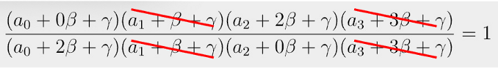
Because β and γ are random, it is practically impossible that the grand product is 1, while the permutation check fails. That is, if a0 != a2, the equation in Fig. 4 will not hold.
Proof
We provide an informal proof that if grand product is 1, σ(i) = j implies ai = aj. Essentially, the permutation check passes if and only if the grand product is 1.
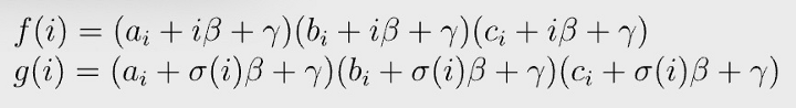
Recall that Schwartz-Zippel lemma says if two polynomials are equal at a random evaluation point, these two polynomials are identical everywhere with overwhelming probability. Let us consider two polynomials.
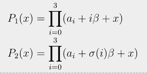
Since they are equal at random γ, we can regard them as the same, meaning they have the same roots.
Consider two matching roots: j-th from P1 and i-th from P2.
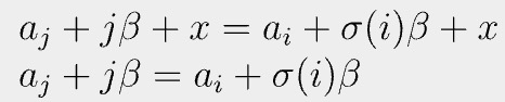
We can apply the trick above again by defining two polynomials:
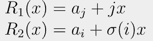
Since they are equal at random β, we can regard them as equal. That is, ai=aj when σ(i) = j. QED[1].
Polynomial
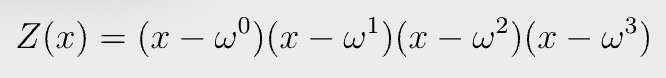
Roots of unity
We used vector index {0, 1, 2, …, n-1} as the domain of evaluation H when converting a vector to a target polynomial, but any domain can be used. In PLONK, the domain that is used for polynomial interpolation consists of roots of unity, due to its performance gains. The n-th roots of unity of a field are the field elements ω that satisfy ω^n = 1. n is the size of the vector, which is 4 in this case. H is {ω⁰, ω¹, ω², ω³ }.
Accumulator
Let us define a vector P evaluated as the following:
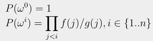
It accumulates the grand product, since P can be rewritten recursively:
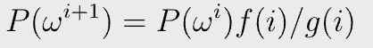
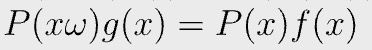
If there exists such as P(x), we know the grand product equation in Fig. 4 holds, since
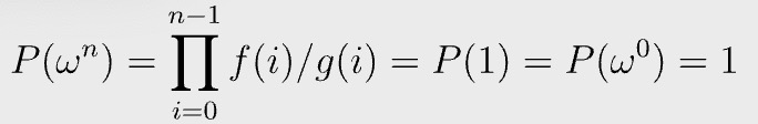
Fig. 7 is equivalent to:
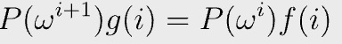
P(x), f(x), and g(x) can be found using interpolation on domain H {ω⁰, ω¹, ω², ω³ } as before. The following polynomial equation holds on the domain H
in which
It is again equivalent to prove the following polynomial equation

in which
We can prove it using a polynomial commitment scheme as in Part 1.
Copy constraints across vectors
There are also copy constraints across different vectors/polynomials, e.g., a2 = b0 and a1 = c0. We can extend the previous method by merging vectors a, b, and c into a single large vector, whose size n is 12. For example, b0 has index 4 and c0 8. The permutation function σ(i) of our toy example becomes:

Fig. 3 becomes:
The remaining steps are similar to the those of enforcing copy constraints within a single vector.
PLONK
To recap, given a program P to prove, we first convert it to an arithmetic circuit, then to a series of constraints including gates and copy constraints, which are transformed into polynomials. Finally, we use a PCS to verify polynomial identities succinctly.
These are all the high-level ideas of using PLONK to prove a computation. We omit a myriad of important optimizations which make PLONK efficient in practice, for ease of exposition. For example, the PCS can be made non-interactive using the standard Fiat-Shamir heuristic. Also testing for multiple polynomial identities can be merged into one. For more details, you can read the original paper or the references below.
References
https://github.com/sCrypt-Inc/awesome-zero-knowledge-proofs#plonk
NOTE:
[1] The proof’s idea comes from here.
Watch: The BSV Global Blockchain Convention presentation, Smart Contracts and Computation on BSV
Recommended for you