How PLONK Works: Part 1

Getting your Trinity Audio player ready...

This post was first published on Medium.

PLONK is a state-of-the-art zk-SNARK proof system. Previous zk-SNARKs such as Groth16 have circuit-specific setup, which requires a new trusted setup for any new circuit. PLONK’s trusted setup is universal, meaning it can be initiated once and reused by all circuits[1]. It is also updatable: one can always add new randomness until one is convinced the setup is not compromised.

This article will explain the core ideas on how to prove a computation using PLONK. The figure below illustrates the steps to take in order to prove a computation using PLONK.

We will explain each step in details.

Arithmetic circuit

PLONK does not understand a program one wants to prove. It first has to be converted to a format called an arithmetic circuit. Arithmetic circuits are circuits made out of two types of gates: addition and multiplication.

Suppose we want to prove we know the solution to the equation P(x) = x³ + x + 5 = 35 (the solution is 3). We can convert it to the following circuit.

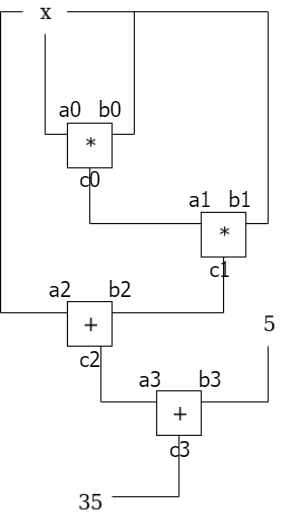
Constraint system

Next, we transform an arithmetic circuit into a constraint system. There are two categories of constraints on the circuit wires.

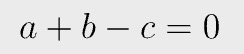
1. Gate constraints

These are constraints within each gate of a circuit. The above circuit has four gates and the following constraints, i.e., equations with a certain format.

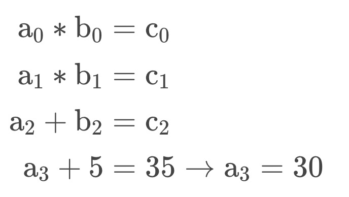
In PLONK, all constraints are normalized/standardized into the following form[2]:

a, b, c are left, right, and output wire of a gate. All Qs are constants.

It can be regarded as a generalized gate, which can be configured by tweaking Qs. For example, setting Qs as follows turns the generic gate into an addition gate.

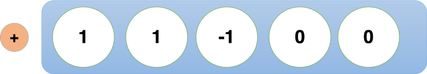
To see how, we set QL = 1, QR = 1, QO = -1, QM = 0, QC=0, Fig. 3 becomes

Similarly, the following configuration represents a multiplication gate.

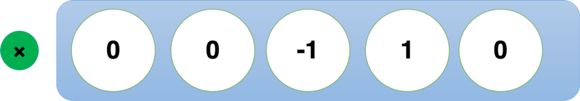
Fig. 2 is normalized to the following:

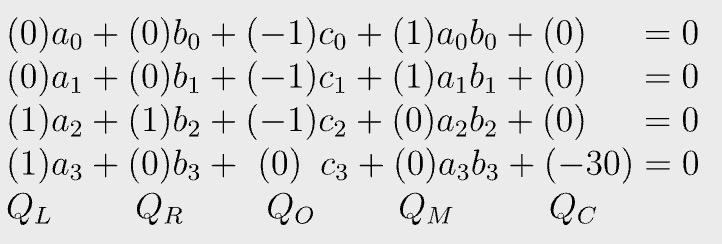
We can rewrite Qs in vector forms:

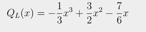
QL​=(0,0,1,1), QR​=(0,0,1,0), QO​=(−1,−1,−1,0), QM​=(1,1,0,0), QC​=(0,0,0,−30).

The Q vectors are called selectors and encode the circuit structure, i.e., the program.

Similarly, we can collect all a, b, and c’s into vectors:

a = (a0, a1, a2, a3), b = (b0, b1, b2, b3), c = (c0, c1, c2, c3).

These vectors are called witness assignments and represent all wire values derived from user inputs, some of which may be private and only known by the prover.

2. Copy constraints

These are constraints across different gates, e.g., c0=a1. We will defer to Part 2 to explain it.

Polynomials

We can turn a vector into a list of points by using its index as the x-coordinate. For example, QL can convert to (0, 0), (1, 0), (2, 1), and (3, 1). There is a unique degree-3 polynomial passing through these points. {0, 1, 2, 3} is called the evaluation domain. QL is in “evaluation form,” while its “coefficient form” can be obtained using interpolation[3].

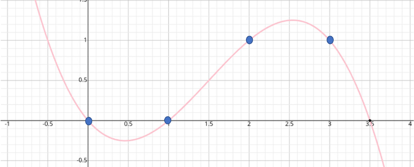
Likewise, we can convert other vectors to polynomials, evaluated at the same domain. Let us define f(x) to be:

f(0) evaluates to 0, since

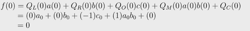
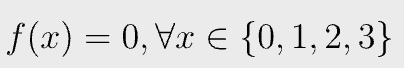
Similarly, you can evaluate f at 1, 2, 3, which all result in 0.

All the constraints in Fig. 7 will be met if and only if the following holds:

We have compressed all constraints to a single polynomial f(x), which can be expressed as follows.

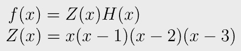
This is because 0, 1, 2, and 3 are roots of f(x). Fig. 9 holds as long as there exists such polynomial H(x) that makes f(x) divide Z(x) without any remainder. Z(x) is called the vanishing/zero polynomial, H(x) the quotient polynomial.

We can define another polynomial g(x):

We only need to show g(x) is 0 everywhere, i.e., it is a zero polynomial.

Schwartz-Zippel lemma

Schwartz–Zippel lemma states: let f(x) be a non-zero polynomial of degree d over a field F of size n, then the probability that f(s) = 0 for a randomly chosen s is at most d/n​. Intuitively, this is because f(x) has, at most d roots. In practice, d is usually no larger than 100 million, while n is close to 2²⁵⁶, meaning d/n = 1/10⁶⁹.

This means if we evaluate polynomials at some random point and the evaluation is 0, it suggests that the polynomials are, in fact, zero everywhere with overwhelming probability.

A corollary is if we evaluate two polynomials at some random point and they are equal, they are equal everywhere almost surely.

Polynomial commitment scheme

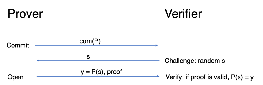
To prove a polynomial P(x) is 0, we use a polynomial commitment scheme (PCS). A PCS can be regarded as a sort of “hash” of some polynomial P(x), and the committer can prove that P evaluates to a certain value at a certain point through a proof without revealing the polynomial P.

A PCS consists of three rounds between a prover and a verifier:

1. Commit: a prover commits to a certain polynomial P and sends it to a verifier
2. Challenge: the verifier wants to evaluate P at a random point s and sends it to the prover
3. Open: the prover evaluates P at s and sends back the result y, along with an evaluation proof. The verifier checks the proof, and if it is valid, he concludes P(s) = y. The polynomial equation itself is efficiently verified by evaluating at a random value.

We can use PCS to prove g(x) is zero in Fig. 11. The PLONK paper uses Kate commitments based on pairing. Other PCSs can be used as well.

We will cover the remaining copy constraint part in the next article. Stay tuned. Please let us know if there is any error.

References

https://github.com/sCrypt-Inc/awesome-zero-knowledge-proofs#plonk

[1] As long as the new circuit is not bigger than the original circuit.

[2] The Plonk constraint system is similar to the rank-one constraint system (R1CS) in that they both can have only one multiplication in each gate. The difference is that R1CS allows unlimited additions in a gate, while Plonk can only do one, excluding the addition of a constant.

[3] In practice, the coefficients will all be integers since all operations are done not over integers but a prime field.

Watch: The BSV Global Blockchain Convention presentation, Academic Accreditation & Certification on the BSV Blockchain